

Expanding Awareness of Public Pension Issues
Showing posts with label Investors. Show all posts
Showing posts with label Investors. Show all posts
Thursday, February 25, 2021


Thursday, October 29, 2020
Investment Indices: The Inside Story

Both the Dow Jones Industrial Average and the S&P 500 Index Have Recently Made Changes. What Does That Mean for Retirement Investors?
Tuesday, August 25, 2020
The Case for a Permanent Allocation to an Equity Stabilization Strategy
 |
| Image by Samuel F. Johanns from Pixabay |
By CRAIG STAPLETON & JEREMY GOGOS/Securian Asset Management
Key Points
- Institutional investors face a balancing act between two equally important needs: achieving robust long-term returns while avoiding the painful consequences of near-term drawdowns.
- Traditional asset allocation, risk parity and other hedging strategies have failed to perform as expected during recent downturns. Fixed income assets have moved closely in line with equities in times of crisis.
- Equity volatility levels exhibit a persistent and reliable relationship with equity returns over time and through market cycles, including the latest market crisis, as illustrated for large cap U.S. equities in Chart 1.
- A permanent strategic allocation to an equity stabilization strategy that utilizes the persistent volatility/return relationship can improve investors’ long-term risk/return ratios – even if implemented right after a market selloff. A rules-based approach, using the reliable indicator of recent volatility, can be successfully applied at any time via a spectrum of implementations against single or multiple risk asset class portfolios.
Chart 1: There is a Clear Relationship Between Monthly Equity Returns and Recent Volatility
Average Monthly S&P 500 Returns for Ranges of Realized Monthly Volatility(January 1, 1928 – March 31, 2020)
 |
Click chart to enlarge. Source: Bloomberg. Data as of April 1, 2020. The data spans from January 1, 1928, to March 31, 2020, and the table displays the average monthly returns for the S&P 500® for the time periods shown where the average monthly volatility was in the different volatility categories shown. Volatility is measured as the annualized standard deviation of daily returns of the index. The S&P 500® Index is an unmanaged index of 500 stocks that is generally representative of the performance of larger companies in the U.S and investments cannot be made directly in the indices. See additional disclosures at the end of the materials for additional information. |
Risk Assets: Investors Manage a Double-Edged Sword
Institutional investors face the pernicious dilemma of having mutually conflicting needs. When building a portfolio, investors start with the understanding that, over the long term, expected return and volatility are strongly positively correlated. Unfortunately, most investors need both significant levels of return to meet their long-term goals and a stable stream of returns to ensure financial viability. A defined benefit pension plan, for example, needs solid returns to meet its actuarial funding goals and pay pensions, while it needs stability to avoid erosion of its funded status.
For institutional investors seeking stable funding, the same risk assets that provide essential upside potential also represent significant exposure to downside risk and unstable results. Although investors’ need for risk mitigation is high, most investors have not implemented such strategies to date, for reasons we discuss below.
The Risks of Managing Risk: Why Most Portfolios Remain Exposed
For a risk mitigation strategy to be reliable, it must be built on a market relationship that is persistent over time. Unfortunately, most risk mitigation strategies to-date have been based on historic correlations that have broken down during strong bear markets, when they are most needed.
Fixed Income is an Anchor to Windward Until a
Hurricane Comes
Unfortunately, the correlation between fixed income and equity investments is not stable through time. As Chart 2 illustrates, there have been long periods where equities and bonds were positively correlated, and thus traditional portfolio diversification did not reduce portfolio risk.
Chart 2: Fixed Income is Not a Reliable Equity Hedge
3-Month Rolling Correlation – S&P 500 and Bloomberg Barclays U.S. Aggregate Bond Index(January 1, 1989 - March 31, 2020)
 |
| Source: Bloomberg Barclays US Aggregate Bond Index and Securian Asset Management, Inc. Data as of April 1, 2020. The data spans from January 1, 1989, to March 31, 2020, and displays analysis of two indices, the 3-month rolling correlation of the S&P 500 vs. the Bloomberg Barclays U.S. Aggregate Bond Index. The blue circles highlight the specific periods of time. Click chart to enlarge. |
In crises — when an offset to downside equity risk is most needed — equities and fixed income often sell off at the same time. During the COVID-19 crisis, the correlation between fixed income assets and equities quickly became much less negative, diluting fixed income’s portfolio diversification benefit. Further, there have been extended periods of time where fixed income was positively correlated with equity. Both are highlighted in the circles in Chart 2.
Volatility is a Reliable Indicator of Equity Performance
A persistent and reliable relationship exists between 1-month volatility and 1‑month equity returns, both positive and negative. Volatility episodes tend to demonstrate persistence. As Chart 3 clearly shows, since 1928, for the S&P 500, high 1-month volatility tends to be associated with poor 1-month returns; and vice versa.
Chart 3: Since 1928, Volatility Levels Have Reliably Signaled Equity Returns
Average Monthly S&P 500 Return vs. Average Monthly Realized Volatility
(January 1, 1928 - March 31, 2020)
 |
Source: Bloomberg, Securian Asset Management, Inc. Data as of April 1, 2020. Data spans from January 1, 1928, to March 31, 2020, and displays the average monthly S&P 500 return vs. the average monthly realized volatility. Click chart to enlarge. |
While we use the S&P 500 for the illustration above, our research shows the same relationship between volatility and returns across other equity markets.
Volatility-Based Equity Stabilization Strategy Can Improve the Risk/Return Ratio
A strategy based on the reliably strong relationship between equity volatility and returns is well-suited to deliver portfolio risk mitigation in a more consistent manner than traditional asset allocation. An Equity Stabilization Strategy systematically adjusts equity exposures based on the volatility/return relationship. This approach holds greater equity market exposure during lower volatility periods, which tends to lead to better performance, as illustrated in Chart 3. Conversely, we believe this approach can quickly reduce equity market exposure during the higher volatility periods that tend to produce unfavorable performance, mitigating the drawdown of assets.
The Case for a Permanent Strategic Portfolio Allocation to Volatility-Based Equity Stabilization Strategies
To-date, institutional investors have implemented volatility-based stabilization strategies sporadically or not at all. We believe this reticence is due to two key investor concerns: Portfolio risk hedging is complex, and a desire to avoid periodic carrying costs of hedging – particularly right after a major market selloff.
A permanent strategic allocation to a systematic volatility-based approach over a full market cycle addresses both of these issues.
A simple set of rules using 1-month risk asset volatility as the principal metric is the foundation of an equity stabilization strategy. A strategic overlay primarily employing listed equity index futures ensures transparency and simplicity while avoiding counterparty risk.
Implementing Volatility-Based Risk Mitigation is Straightforward
The Stabilized Equity Portfolio Hypothetical Example, is based on a pension plan aiming to reduce its domestic U.S. equity annualized volatility by about 25% from its historic average level of around 18% per annum. In this hypothetical, the pension fund added a futures-based overlay on top of its equity portfolio, using listed S&P 500 futures to dial the effective equity exposure up or down based on volatility. Using this overlay, the portfolio manager allows the portfolio’s effective equity position to drop down to 20% of the portfolio’s net assets in high volatility environments and increase it to as much as 150% in low volatility environments.
Chart 4: Equity Stabilization Strategy Improves Risk/Return
Stabilized Equity Portfolio Hypothetical Risk & Return
(January 1, 1988 - March 31, 2020)
 |
| Source: Bloomberg, Securian Asset Management, Inc. The data spans from January 1, 1988, to March 31, 2020, and displays the hypothetical backtested returns of a hypothetical portfolio created for illustrative purposes only. No investor actually achieved the results shown. No representation is being made that any account will or is likely to achieve results similar to those shown. Please see important disclosures on the limitations of hypothetical backtested performance at the end of the materials. Click chart to enlarge. |
Skillful Implementation Adds Further Value to a Stabilization Strategy
The pension fund’s overlay manager should take the following steps:
- Run the overlay model daily
- Combine experience-based judgement and additional subsidiary indicators such as the VIX and high-yield spreads to better assess the likely volatility environment daily
- Primarily use listed futures, and use listed options when inexpensive or more attractive
- Employ strict trading rules to protect the pension fund from being whipsawed in rapidly changing market environments
- Employ strong derivatives governance and oversight
Balanced Portfolios Benefit as Well
Using a volatility-based risk mitigation strategy on the equity portion of a balanced portfolio is an effective way to adjust the equity/bond mix to changing risk environments, without the costs and timing issues of selling the underlying assets.
Positive Full Market Cycle Cost/Benefit
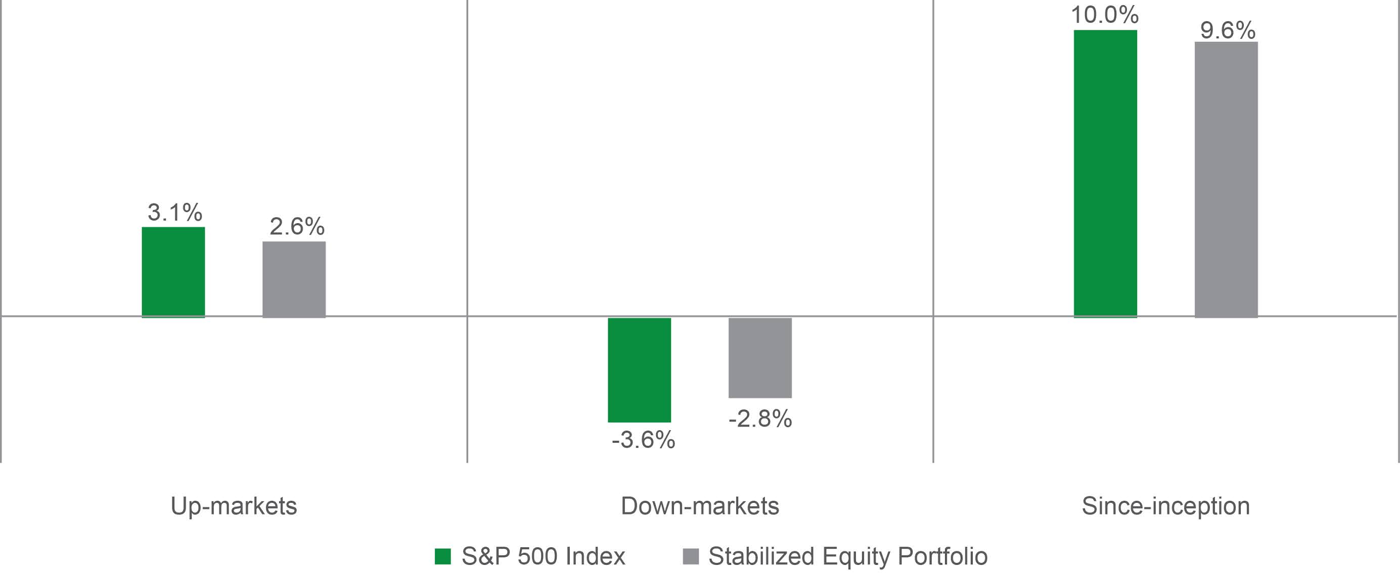
When a volatility-based portfolio risk management approach is maintained throughout a full market cycle, its outperformance in down markets can offset its underperformance in up markets, rendering a market-like return over a full cycle.
Chart 5: Thoughtful Equity Stabilization Can Pay for Itself Over a Full Market Cycle
Average Monthly Returns of the S&P 500 Index and the Stabilized Equity Portfolio Hypothetical Example in Up Markets, Down Markets, and Longer-term
(January 1, 1988 - March 31, 2020)
 |
| Source: Bloomberg, Securian Asset Management, Inc. The data spans from January 1, 1988, to March 31, 2020, and displays the hypothetical backtested returns of a hypothetical portfolio created for illustrative purposes only. No investor actually achieved the results shown. No representation is being made that any account will or is likely to achieve results similar to those shown. Please see important disclosures on the limitations of hypothetical backtested performance at the end of the materials. Click chart to enlarge. |
Implementing a volatility-based risk mitigation approach by means of a derivative overlay means there is no disposition of underlying assets, merely a modification of risk exposures, thus avoiding trading costs and buy/sell spread costs. While there may be periodic ‘carrying costs’ of foregone performance in a bull market, the strategy tends to pay for itself over a full market cycle – avoiding the extensive long-term portfolio damage that a liquidity crisis during a bear market can wreak – as shown in Chart 5, above.
Portfolio Hedging is Vital after a Market Selloff
Perhaps counterintuitively, a volatility-based stabilization strategy is vital after a severe market shock, such as the recent COVID-19 pandemic shock.
After an historic downturn in the markets, most institutional portfolios are significantly underweight equities. In order to benefit fully when the markets inevitably recover – and in order to rebalance to their strategic asset mix targets – institutions need to re-risk by adding to their equity exposures.
This may be a difficult decision for many institutions, because the market bottom is only known to have occurred well after the fact. A reliable risk management strategy, such as the kind of volatility-based approach described in this paper, enables institutions to re-risk without needing to have certainty about the market bottom, as it entails significant protection against further drawdowns and yet will participate when the market recovers.
Summary: A Permanent Allocation to Volatility-Based Risk Mitigation is a Strategic Necessity for Institutional Investors
An airbag must be permanently installed in a car in order for it to deploy when it is needed – during the moment of impact, the timing of which cannot be predicted.
Similarly, we believe institutional investors obtain the best results from a stabilization approach based on volatility when they make it a full-time strategic allocation in their portfolios. A permanent strategic allocation to volatility-based stabilization ensures investors and their beneficiaries can benefit from the consistent and sustained mitigation of volatility shocks on an ongoing basis.
Securian Asset Management is an Associate Member of TEXPERS. The views expressed in this article are those of the authors and not necessarily Securian Asset Management nor TEXPERS.
About the Authors
Craig Stapleton, CFA, FRM is Senior Vice President – Head of ALM & Quantitative Strategies at Securian Asset Management. As Vice President and Portfolio Manager, Stapleton is responsible for derivatives, agency MBS, government and municipal bonds, quantitative analytics, cash management, ALM and strategic asset allocation for the Minnesota Life General Account. He is the head of the quantitative analysis and research group. Stapleton is also the co-portfolio manager for the Equity Stabilization strategies and the Securian Asset Management Strategic Dividend Income portfolios. Prior to his role as portfolio manager, Stapleton provided quantitative analysis, security and portfolio risk statistics, and derivatives hedging capabilities for Securian Asset Management and its clients. Stapleton is a CFA Charterholder, and a member of the CFA Institute and CFA Society of Minnesota.
Jeremy Gogos, Ph.D., CFA, is Vice President and Portfolio Manager of Quantitative Strategies at Securian Asset Management. He monitors domestic and international equity volatility and correlation, manages fund equity exposure, and evaluates equity allocation model performance. Gogos provides quantitative analysis, security and portfolio risk statistics, and execution of derivative and hedging initiatives. He has also supported annuity, life insurance, and investment product designs with stochastic and historical simulation and performance evaluation. Prior to joining Securian Asset Management, Gogos was a computer programmer supporting Securian Retirement’s 401(k) recordkeeping and trading platforms. He is a CFA Charterholder, and is a member of the CFA Institute and CFA Society of Minnesota.
Friday, June 21, 2019

BY PHIL DESANTIS, Westwood Holdings Group
As a high-performing equity market environment lifted most stocks over the last decade, the value proposition for active management in efficient asset classes such as U.S. Large Cap has been scrutinized by both institutional and retail investors alike.
Low active share, otherwise known as “closet indexing,” high turnover and lofty management fees all contributed to a trend of marginal performance results for active products relative to benchmarks. In response, many investors have chosen to reduce their allocations to active managers and increase passive holdings, particularly in efficient asset classes.

During this period of dominance by passive products, the relationship between asset owners and investment managers has transformed, increasing fee pressures to improve alignment over existing fee structures. While overall fees have come down over the last decade, the industry has done very little to truly level the playing field for investors and solve the real problem — aligning fees to the value of active management and improving the probability of a favorable outcome depending on manager skill and the efficiency of the asset class.
Mutual fund investors paid a staggering $100 billion dollars in expenses to underperforming asset managers over the last ten calendar years.
We believe the industry is primed for a major disruption that will better reflect the value- added returns of active management by solving the fee problem, altering the probability of winning for investors, and in turn radically changing asset allocation decisions.
Read more in our whitepaper, “Mission Possible: Changing the Probability of Winning for Active Investors.”
The views expressed herein do not constitute research, investment advice or trade recommendations, do not necessarily represent the views of Westwood Holdings Group nor TEXPERS, and are subject to revision over time.
About the Author:


BY MARK SHORE, Coquest Advisors
Investment volatility, or “vol,” as it is known on the street, is often measured by the standard deviation. Investors frequently use the standard deviation as a proxy for risk. But is the standard deviation a proxy for risk or a proxy for dispersion around the mean?
Investors often talk about volatility when portfolios are losing value. For example, you probably won’t hear much discussion about the stock market being volatile when it rallies. That discussion usually occurs when stocks decline. However, when an investment has profitable returns, it is still technically defined as volatility, sometimes known as upside volatility or positive volatility. Investors are usually accepting of the upside vol, as it implies the investment experiences positive returns. It’s the downside vol investors are often losing value as that is the tail risk they are usually trying to reduce. To paraphrase from my paper, Skewing Your Diversification, volatility is comparable to cholesterol. There is good and bad volatility.
The traditional view perceives higher standard deviation equating to higher risk. But is that always the case? As I often tell the students in my managed futures class, you should understand if the volatility derives more from the positive returns or the negative returns. If derived more from the positive side of the distribution, that is the dispersion of the positive gains that is inflating the standard deviation. If the volatility is derived more from the negative volatility than it is the dispersion from the negative returns and is the tail risk, that usually concerns investors.
Modern portfolio theory assumes a normal return (bell-shaped) distribution. However, distributions may be skewed (asymmetrical curve) to the right causing positive volatility or skewed to the left, causing negative volatility. The negatively skewed distribution may cause increased tail risk and losses, as noted in the chart below.

Understanding how an investment’s allocation impacts the portfolio’s skewness helps understand the behavior of the allocation relative to the portfolio. Does it expand the skewness to the left or the right? This concept is also known as co-skewness, according to the authors of Conditional Skewness in Asset Pricing Tests, published in The Journal of Finance.
In other words, an investment with a high standard deviation but more volatility coming from the upside could potentially reduce a portfolio’s volatility when the investment is allocated to a portfolio. It sounds counter-intuitive for a high standard deviation investment to reduce a portfolio’s standard deviation, but it’s the positive volatility that is offering the benefits to the portfolio to reduce the tail risk and downside vol.
An investment with a high standard deviation derived from positive skewness and coupled with a low or non-correlation to the portfolio may increase the added value of the allocation. It’s also possible for an investment with a low standard deviation, but more volatility attributed to the downside increasing the portfolio’s tail risk.
Therefore, only accounting for a standard deviation to be high or low is not enough. Drilling down to understand where the volatility is good or bad is an essential factor to consider. If the tail risk can be more efficiently controlled, than the portfolio’s drawdowns may also be reduced.
The views expressed herein do not constitute research, investment advice or trade recommendations, do not necessarily represent the views of Coquest Advisors nor TEXPERS, and are subject to revision over time.
 About the Author:
 Mark Shore is the director of educational research at Coquest Advisors. He is also an adjunct professor at DePaul University. He is a candidate to receive his doctorate in business administration in 2020. He has a master's degree in finance from The University of Chicago Booth School of Business. He also has a bachelor's degree in finance from DePaul University.

BY JIM MCKEE, Callan
Looking for improvement from your hedge fund allocation? Co-investing with hedge funds is a chance for investors to enhance returns while reducing overall fees.
Although co-investments have been a popular supplement to a fund sponsor’s private equity and real estate programs for decades, co-investing with hedge fund managers became a widespread practice only after the global financial crisis of 2007-2008.
The appeal of co-investing with hedge funds today arises from attractive opportunities that lie between the vast pools of liquid capital markets dominated by algorithms and indexers on one side, and the mountain of dry powder controlled by private equity providers on the other.
What are co-investments?
Co-investments are one-off investments that a hedge fund manager has identified which are typically too illiquid or oversized to absorb within the manager’s flagship fund. Another key feature of such opportunities is that they need to be assessed quickly for a decision to buy or pass—often within days or weeks.Fast-moving markets or events are frequently forcing the trade; being able to respond within a few days or weeks is the key for successful participants. Because market values of such opportunities are often not observable due to their size or illiquidity, the allure for co-investors is an asset trading at a notable discount to fair value, in addition to lower fees charged by the sourcing manager versus its commingled fund vehicle.
What have co-investments looked like in the past?
Depending on the manager’s domain expertise, they could be Lehman claims, Icelandic bank debt, Puerto Rican bonds, Argentinian debt, Egyptian T-bills, CLO equity tranches, late-stage private equity, or an activist-controlled stake in a targeted public stock. Other investment opportunities may not be co-investments, per se, but are similarly attractive to experienced buyers looking for direct investments offered by motivated sellers at a material discount, such as hedge fund secondaries.Motives behind offerings
Motives behind managers offering co-investments are many. In addition to a position being too big or too illiquid for their primary commingled fund, co-investments represent an opportunity to create and improve relationships with strategic clients while developing a supplemental revenue base. Since co-investments are usually offered under carefully described circumstances, investors in such opportunities should not construe them as the manager’s “best ideas”—one should expect those to continue going first into the manager’s flagship fund.Investor expectations
Since co-investments are offered at lower fees, the investor’s expectation should be to improve performance at least by reducing the fees being charged. A collateral benefit is that co-investing efforts provide improved access to deal flow via dedicated sourcing experts. Furthermore, co-investing provides more transparency into a manager’s investment process. Because the manager’s compensation is typically driven by incentive fees, the investor can also be more confident in aligned interests to create desired investment outcomes. Nevertheless, working with multiple co-investing partners helps to improve diversification of trade risks.Because resources and experience widely vary among investors, co-investment solutions have three primary forms to consider:
- If limited partners lack resources to quickly vet and approve opportunities presented to them, they can consider a turnkey solution provided by a fully discretionary adviser, whether a hedge fund or fund-of-funds manager. The adviser of this turnkey solution sources the co-investment deals, underwrites them, and uses its full discretion to implement a commingled fund solution. It is the most fee-laden solution, but it is cheaper than the manager’s full-fee commingled fund.
- Limited partners with demonstrated experience and ability to move quickly on any presented opportunity can oversee a managed account of approved co-investments that conforms to customized investment guidelines set up with the manager.
- If an investor has significant size, experienced staff, and demonstrated resources, it can be a strategic partner working with manager sourcing, vetting, and investing directly in deals.
The views expressed herein do not constitute research, investment advice or trade recommendations, do not necessarily represent the views of Callan nor TEXPERS, and are subject to revision over time.
 About the Author:
 Jim McKee is a senior vice president in Callan's Hedge Fund Research group. He is a shareholder of the firm. McKee earned a master's degree in finance from Golden Gate University in 1987. He received his bachelor's degree in economics/environmental studies from Dartmouth College in 1982.

The yield curve simply tracks how long-term interest rates stack up to short-term rates, and it’s said to invert when short-term rates are higher than long-term ones. After three-month Treasury bill rates topped those of 10-year Treasury yields for the first time since 2006, we took a closer look at what happened to equity returns after the 11 other inversions that have occurred since the 1960s.
In the very short term, the effect of an inversion is negative. In recent years, that may be because the yield curve has gained incredible power in the minds of financial market participants as a foolproof signal of impending recession. In other words, the signal itself, rather than any fundamental conditions it signifies, might make investors nervous. In earlier years, when yield-curve inversions didn’t even warrant a mention in the New York Times, concern over how rising short-term interest rates would affect loan conditions seemed to be more top of mind.
However, average stock returns were negative only in the first month after an inversion. Further out, average returns were positive. And the more time that elapsed since the inversion, the more positive the average returns were.
Looking more closely at long-term trends, however, the picture is more nuanced. Three months after an inversion, stock investors booked positive returns nearly three-quarters of the time. But by the time a year had passed, the results were usually much more extreme: either very positive or very negative.
 |
| Click chart to enlarge. |
What’s the Central Bank Got to Do with It?
The Federal Reserve may have contributed to those extreme results. During the three best yearlong periods of post-inversion returns, with gains ranging from 27.1% to 33.6%, the Fed was generally in loosening mode.On the flip side, the Fed was generally in tightening mode during all but one of the five yearlong post-inversion periods in which investors experienced negative returns. And the one year of negative returns in which the Fed was not strictly tightening, having both raised and lowered interest rates between October 1980 and October 1981, turned out to be the “best of the worst.” The returns of –7.3% that year compare favorably to double-digit losses in other post-inversion periods.
At the moment, the Fed has put further rate hikes on ice, and some investors even believe cuts are in the offing. Historical data reinforce the idea that cutting would likely be better for markets, but the data also show that it’s possible for equity markets to keep going up even under tightening monetary conditions.
Zooming Out: The Bigger Economic Picture
Much depends on the broader economic context in which inversions occurred. For example, when the yield curve inverted in September 1988, the US economy was in its eighth year of expansion. The Asian financial crisis hit many global economies hard, but it failed to slow job creation, arrest the falling unemployment rate or nudge inflation higher in the US. The economy continued to expand into 1999, and US stock investors enjoyed the best returns of all 11 post-inversion periods.The worst post-inversion returns, however, came soon after that period, with the April 5, 2000, inversion. The Fed had hiked interest rates five times since June 1999, unemployment began rising in May 2000 and technology stocks melted down. The disputed presidential election in November 2000 only added to the tumult. The US ended a 10-year run of economic growth with a recession that began in March 2001.
Investors can and will debate whether history will remember 2019 more like 1998 or 2000. And in the late stages of an economic cycle, it’s tempting to let events like a yield-curve inversion influence investment strategy. But we think investors should not be guided by these impulses.
The yield curve is a signal with no precision: though inversions have preceded recessions, they don’t pinpoint when they’re coming. We’ve also never seen an inversion in the post-QE age, and we’re skeptical that it’s a valid signal for equities this time around. Rates are still historically low, global central banks have paused any move toward tightening and some countries are even unleashing fiscal stimulus. This inversion was also quite brief, and the curve has since steepened, making this a faint signal at best.
Perhaps most importantly, however, inversions say very little about the fundamental ability of individual corporations to grow and prosper under a range of economic conditions. That’s why returns at any point after an inversion aren’t reliably positive or negative. Companies with high-quality growth, low leverage and high-rated credit are likely to fare well whenever the cycle finally turns. It’s best to stick with what works for now.
The views expressed herein do not constitute research, investment advice or trade recommendations, do not necessarily represent the views of all AB portfolio-management teams nor TEXPERS, and are subject to revision over time.
 About the Author
Scott Krauthamer is managing director of AB’s equity business development and covers the U.S., international and global services for both its institutional and retail growth products. Prior to joining the firm, he held a variety of investment and product-management roles at Legg Mason, U.S. Trust, Bank of America and J.P. Morgan Private Bank. He holds a bachelor's degree in finance and management information systems from the State University of New York, Albany. He is a CFA charterholder and a CAIA designee.
Subscribe to:
Posts (Atom)